Table of Contents
- Table of Contents
- Introduction
- Frequency in the graph domain
- GSP using the Laplacian
- Graph filtering
- Conclusion
- References
Introduction
In the previous article, we introduced the outlines of an emerging field known as graph signal processing (GSP) by presenting it as a natural extension of classical signal processing techniques onto the domain of graphs. More specifically, we discussed GSP techniques using the graph adjacency, that can be applied to both directed and undirected graphs. Here, we present GSP methods based off the graph Laplacian which–though it can only be applied to undirected graphs–offers better overall performance. We will discuss how frequency is intepreted in the graph domain, the motivation for using the graph Laplacian for the basis of signal processing on graphs, and show how filters can be designed for graphs (with an application-driven example).
For this article, CV2, a computer vision python library, to load and process images. Additionally, SymPy will be used to display formatted matrices automatically.
import cv2
import matplotlib.pyplot as plt
import numpy as np
from sympy import *

# for printing SymPy matrices
init_printing(use_unicode=True)
# for code reproducability
np.random.seed(41)
Frequency in the graph domain
Before discussing signal procesing techniques using the graph Laplacian, we must first motivate it by discussing how frequency is interpreted in the graphic domain. To do this, we will go over the concepts of smoothness and zero-crossings as it pertains to signals on graphs.
Graph smoothness
In the first article, it was shown that for a function $f \in \mathbb{R}^N$ and combinatorial graph Laplacian $L$, the following equation holds true: $f^T L f = \dfrac{1}{2} \sum_{i,j=1}^N w_{ij} (f_i - f_j)^2$. Similarly, for the symmetric normalized Laplacian $\mathcal{L}$, the following holds: $f^T \mathcal{L} f = \dfrac{1}{2} \sum_{i,j=1}^N w_{ij} (\dfrac{f_i}{\sqrt{d_i}} - \dfrac{f_j}{\sqrt{d_j}})^2$. Both of these are a measure of smoothness of the graph, which we will denote as $\lvert \lvert f \rvert \rvert_L$ for a function $f$. Interestingly, if we let $f$ equal the eigenvector of the graph Laplacian $u_k$, the smoothness $\lvert \lvert u_k \rvert \rvert_L = u_k^T L u_k$ gives us the coresponding eigenvalue $\lambda_k$. From this, we can conclude the eigenvalues of the graph Laplacian are a measure of smoothness, or the amount of oscillation on the graph. This gives us a fine graphical analog of frequency. To be more specific, given an eigenvalue $\lambda_k$, small $k$’s measure low frequency components while large $k$’s give higher frequency components. [1]
Zero-crossings
Another useful measure for frequency of a signal on a graph is that of the number of zero-crossings, or the number of positive-valued nodes connected to negative-valued nodes. Mathematically, the set of zero-crossings of a signal $f$ on a graph $\mathcal{G} = (\mathcal{V}, \mathcal{E}, W)$ is given as $\mathcal{Z}_{\mathcal{G}}(f) := { (i, j) \in \mathcal{E}: f(i) f(j) < 0 }$. [2]

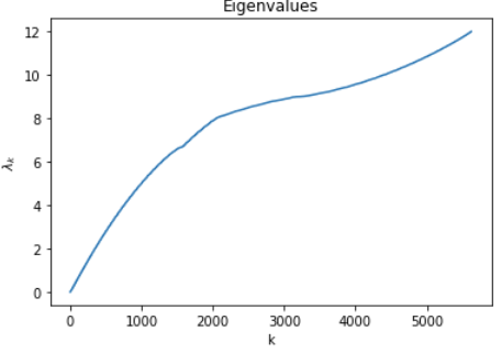
Figure 1: The ordered set of eigevalues is a representation of zero-crossings
GSP using the Laplacian
This article gives a great motivation for why the graph Laplacian is a graphical analog to the time/space domain’s Laplacian operator. In particular, the eigenvectors of the Laplace operator $\nabla$ are the complex exponentials seen in the Fourier transform [3]. Likewise, our graphical analog to the Laplace operator, the graph Laplacian, has eigenvectors that are used in the graph Fourier transform, which is defined as $\hat{f} = U^{-1} f$ where $L = U \Lambda U^{-1}$. Each entry in $\hat{f}$ representes the power at that frequency i.e. $\hat{f}(k) = f^T u_k^*$. Since the graph Laplacian is symmetric, it also holds true that $U^{-1} = U^T$ and that the eigenvalues are real-valued. [2]
On the subject of which graph Laplacian to choose (the combinatorial or symmetric normalized?), the question is still up in the air [2]! In this series–unless stated otherwise–we will use the combinatorial graph Laplacian for its quick and easy computation.
Graph filtering
We will motivate GSP with an application in image processing. More specifically, we will design a filter in the graph domain to remove noise from an image, and compare our result to a standard Gaussian image filter. We start with loading in the famous Lenna photo ubiquitous to image processing, and then convert it into an easy-to-process format by first downscaling and then converting it to a 1-channel grayscale image. Noise is then added to replicate the transmission of the image over a noisy channel such that $\mathbf{y} = \mathbf{x} + \nu$ where $\nu \sim \mathcal{N}(0, \sigma^2)$. [2]
# image parameters
dim = 75
N = dim ** 2
noise_std_dev = 10

# read in image
img = cv2.imread('./path/to/image/here/lenna.png')

# downsample
ds_img = cv2.resize(img, dsize=(dim, dim), interpolation=cv2.INTER_CUBIC)

# convert to gray scale
x = cv2.cvtColor(ds_img, cv2.COLOR_BGR2GRAY)

# add noise
noise = np.random.normal(0, noise_std_dev, (dim, dim))
nu = noise.reshape(dim, dim).astype('uint8')
y = x + nu

# display
plt.figure(figsize = (20,10))
plt.imshow(X, cmap='gray')
plt.title('Noisy Lenna')

Figure 2: The original “Lenna” picture

Figure 3: A significantly distorted version of the “Lenna” picture
Image-to-graph
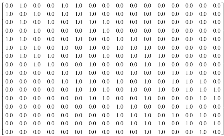
Before doing any GSP, we must first convert the image into a graphical representation. To do this, we will represent pixels by nodes and adjacent pixels by edges [2]. Adjacent pixels are pixels that are to the right, left, top, bottom, or diagonal to the reference pixel. The degree and graph Laplacian are then constructed.
# reshape to vector
y_vect = y.flatten()

# construct graph of image
neighboring_nodes = [-dim-1, -dim, -dim+1, -1, 1, dim-1, dim, dim+1]
W = np.zeros((N, N))
for n in range(N) :
    for i in neighboring_nodes :
        index = n + i
        # check if index in bounds
        if (index >= 0) and (index < N)  :
            # check edge case
            if not (((n % dim == 0) and ((index+1) % dim == 0)) or
                    (((n+1) % dim == 0) and (index % dim == 0))) :
                W[n, n+i] = 1

# construct degree matrix
D = np.zeros(N)
for i in range(N) :
    D[i] = np.sum(W[i, :])

# construct Laplacian
L = np.diag(D) - W

Figure 4: An adjacency matrix for a $4 \times 4$ image
Graph Filter Design
We will first introduce our graph filter design problem as an optimization problem, and then compare the result to its temporal cousin. The problem of estimating our original denoised signal $\mathbf{x}$ from our observed noisy signal $\mathbf{y}$ over the graph represented by the graph Laplacian $L$ is as follows:
$\textrm{arg min}_x \lvert \lvert \mathbf{x} - \mathbf{y} \rvert \rvert_2^2 + \gamma \lvert \vert \mathbf{x} \rvert \rvert_L$ [2]
In a nutshell, the equation wants to minimize the squared error between $\mathbf{x}$ and $\mathbf{y}$ with a regularizing term $\lvert \lvert \mathbf{x} \rvert \rvert_L = \mathbf{x}^T L \mathbf{x}$ of the graph signal’s smoothness [2]. Larger values of $\gamma$ result in a smoother signal, and vice versa. The solution to the above minimization problem is given below:
$\mathbf{x} = h(\lambda) \mathbf{y}$, where $h(\lambda) = \dfrac{1}{1 + \gamma \lambda}$ [2]
It is interesting to note the similrity between our graph filter solution $h(\lambda) = \dfrac{1}{1 + \gamma \lambda}$ and the z-transform of an IIR filter $h(z) = \dfrac{1}{1 - \alpha z^{-1}}$ which acts as a lowpass filter. Like before, we will use the eigendecomposition to compute the filter $h(\lambda)$. This time, however, we will use the SVD to take the eigendecomposition (as it is quicker numerically) and do it on the graph Laplacian instead of adjacency. We will then apply the above equation to the eigenvalues (or singularvalues…) to get our filter output.
# eigen decomposition
U, s, V_T = np.linalg.svd(L, full_matrices=True)

# filter parameters
gamma = 1

# construct filter
h_s = 1 / (1 + gamma * s)
H = U @ np.diag(h_s) @ V_T

# apply filter
x = H @ y_vect

# display result
plt.figure(figsize = (20,10))
plt.imshow(x.reshape(dim, dim), cmap='gray')
plt.title('Graph Filtered Lenna')

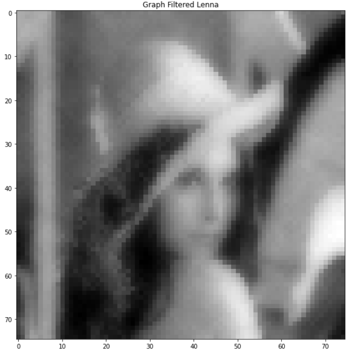
Figure 5: graph filtered image
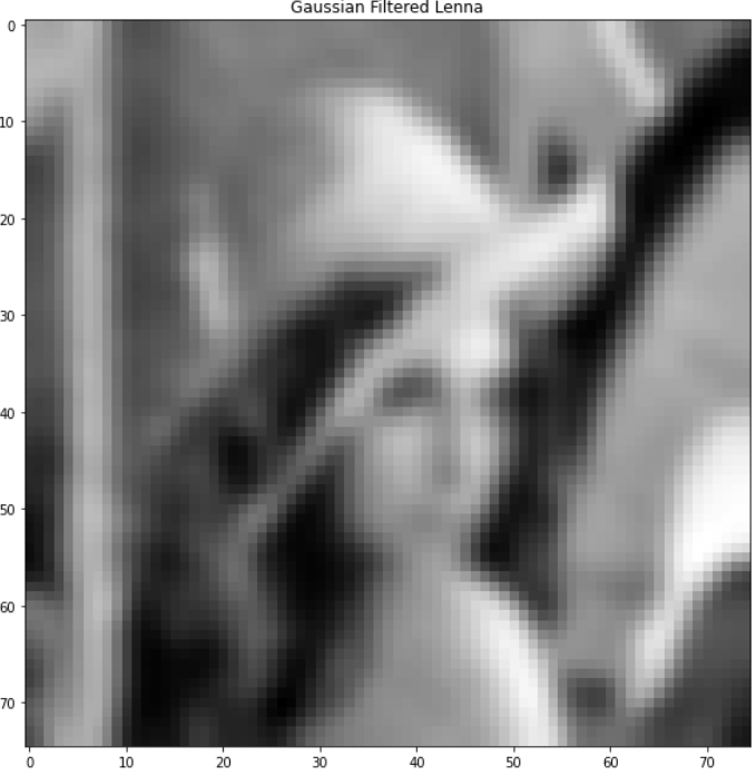
For comparison, here is the Gaussian filtered image:
# Gaussian image filter
x_gf = cv2.GaussianBlur(y, (7,7), 0)

# display result
plt.figure(figsize = (20,10))
plt.imshow(x_gf, cmap='gray')
plt.title('Gaussian Filtered Lenna')

Figure 6: Gaussian filtered image
Filter comparison
The reader will observe that the graph filtered image is much sharper than the Gaussian filter image. This is because the graph filter does not smoothen across the edges of the image as this is encoded within the graph Laplacian, resulting in a less “smeared” output. It is worth mentoning that the graph filter took much longer to compute. Namely, the eigendecomposition/SVD takes significant computation time as it must decompose a matrix of several thousand values. This is a significant downside to GSP as nearly all algorithms employ some decompostion of either the adjacency or graph Laplacian. One of the big open areas of research in GSP is finding cost-effective approximations to these solutions. [2]
Conclusion
In this article, we have extended the GSP framework we developed previously to graph Laplacians, which are typically known to perform better in practice. The ideas of smoothness and zero-crossings are discussed as they pertain to characterizing graph signal frequencies. Using the application of image denoising, we show that GSP can significantly outperform traditional filtering techniques in terms of reconstructing a distorted image, but falls short in ease and cost of computation.
References
[1] Stanković, Ljubiša, Miloš Daković, and Ervin Sejdić. “Introduction to graph signal processing.” Vertex-Frequency Analysis of Graph Signals. Springer, Cham, 2019. 3-108.
[2] Shuman, David I., et al. “The emerging field of signal processing on graphs: Extending high-dimensional data analysis to networks and other irregular domains.” IEEE signal processing magazine 30.3 (2013): 83-98.
[3] Kun, Jeremy. “What’s up with the Graph Laplacian?” 20 Sept. 2016, https://samidavies.wordpress.com/2016/09/20/whats-up-with-the-graph-laplacian/.
