Table of Contents
- Table of Contents
- Introduction
- Matrix representations of DSP operators
- Defining signal processing on graphs
- Conclusion
- References
Introduction
Graph Signal Processing (GSP) is an emerging field that generalizes DSP concepts to graphical models. Here, we review how linear algebra can be used to represent classical DSP operations, and then generalize these operations to signals on graphs. More specifically, we discuss GSP using graph adjacenecy matrices and how a cyclic graph is a graph-theoretic representation of the time domain common in DSP. For background on graph theory, I refer the reader to the previous page Graph Theory and Linear Algebra. The aforementioned article goes over why graphs are a useful representation for data (even data you may not initially think of as a graph), special matrices used to represent graphs, and an introduction to spectral graph theory.
For this article, we will use PyGSP, a graphical signal processing library, to create and display graphs (Note that much of the functionallity appears to be different than the documentation). Additionally, SymPy will be used to display formatted matrices automatically. SciPy is used to compute the DFT.
import matplotlib.pyplot as plt
import numpy as np
from pygsp import *
from scipy.fft import fftfreq
from sympy import *

# for printing SymPy matrices
init_printing(use_unicode=True)
# for code reproducability
np.random.seed(42)
Matrix representations of DSP operators
Vector spaces and, by extension, linear algebra offers a convenient framework for digital signal processing (DSP). This section will use Vetterli et al.’s Foundations of Signal Processing [1] as a reference to review matrix representations of several commonly used operators in DSP.
Signal
Any 1-D discretely sampled signal can be represented as a vector $\mathbf{x} = [… \; x_{-2} \; x_{-1} \; x_{0} \; x_{1} \; x_{2} \; …]^T$. Typically, due to computational constraints, we only look at a finite window of the signal at any given time. This induces a finite dimensioned vector space $\mathbf{x} \in \mathbb{C}^N$ such that $\mathbf{x} = [x_0 \; x_1 \; … \; x_{N-1}]^T$. Likewise, a 2-D signal can be represented by the vector space $\mathbf{x} \in \mathbb{C}^{N \times M}$ such that $\mathbf{x}$ is a matrix. Although this initially may be seen as a convoluted way to represent an array of samples, this definition allows us to apply linear algebra to represent operators and transformations commonly used to process discrete signals. [1]
# signl parameters
N = 40  # number of samples
f0, f1 = 100, 800  # signal frequency
A0, A1 = 1, 0.3  # signal amplitude
fs = 4000  # sampling frequency

# define signal
n = np.arange(0, N)
t = n / fs
x = A0 * np.sin(2 * np.pi * f0 * t) + A1 * np.sin(2 * np.pi * f1 * t)

# display signal
plt.stem(t, x)
plt.ylabel('x')
plt.xlabel('t')
plt.title('Signal')
plt.show()
The above code generates the following (truncated) vector and plot, respectively:
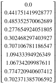
Figure 1: Truncated vector representing signal
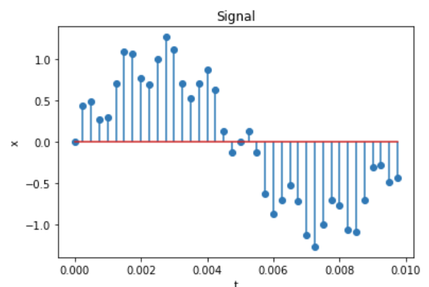
Figure 2: Plot of signal
Time shift
For the following operations/transforms, we will use the same setup of constructing a matrix $A \in \mathbb{C}^{N \times N}$ that transforms the signal into another representation or domain. For each operator/transform $A$, the output is computed by the simple matrix multiplication $\mathbf{y} = A \mathbf{x}$. The simplest operation one can perform on a signal is the time shift, which outputs the previous sample. This has a difference equation of $y_n = x_{n-z}$, where $z \in \mathbb{Z}$ is the number of samples to shift by [1]. Code to construct a time shift matrix is shown below.
# shift count
z = 1

# construct shift matrix
A = np.zeros((N, N))
for i in range(N-z) :
    A[i+z, i] = 1

# perform shift operation
y = A @ x

# display result
plt.stem(t, x, 'b', markerfmt='bo', label='original')
plt.stem(t, y, 'r', markerfmt='ro', label='shifted')
plt.ylabel('x')
plt.xlabel('t')
plt.title('Shifted Signal')
plt.legend()
plt.show()
Below is a truncated version of the shift matrix. Note that this shift by $1$ is simply the diagonal of the identity matrix shifted to the left by $1$.
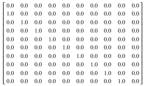
Figure 3: Truncated version of shift matrix
As can be seen below, the output $y_n$ is a shifted version of $x_n$.
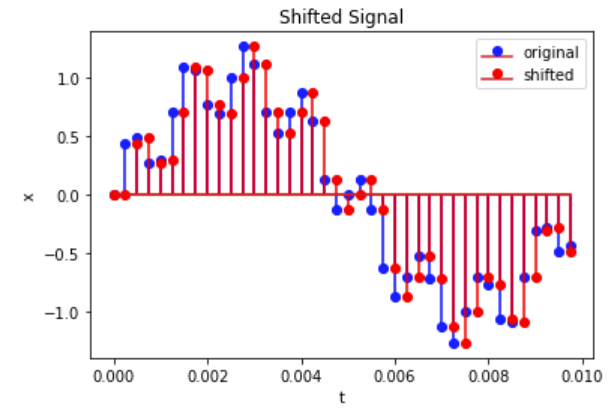
Figure 4: Plots of original and shifted signals
Filter
We will next look at how to construct the filter operator by looking at one of the simplest filters: the moving-average (MA) filter. A moving average filter of length $L \in \mathbb{Z}$ is defined by its difference equation $y_n = \dfrac{1}{L} (x_{n} + x_{n-1} + … + x_{n-L+1})$ [1]. Code to construct a causal MA filter is shown below.
# define MA filter
L = 5
taps = (1 / L) * np.ones(L)


# construct filter matrix
H = np.zeros((N, N))
for i in range(N-L) :
    for j in range(L) :
        if (i-j >= 0) :
            H[i, i-j] = taps[j]

# perform filtering operation
y = H @ x

# display result
plt.stem(t[:-L], x[:-L], 'b', markerfmt='bo', label='original')
plt.stem(t[:-L], y[:-L], 'r', markerfmt='ro', label='filtered')
plt.ylabel('x')
plt.xlabel('t')
plt.title('Filtered Signal')
plt.legend()
plt.show()
Below shows a truncated version of the filter matrix $H$. Filter matrices are Toeplitz (that is, constant along the diagonals), and causal filter matrices are lower trianglular (the matrix has non-zero elements only at or below the diagonal).
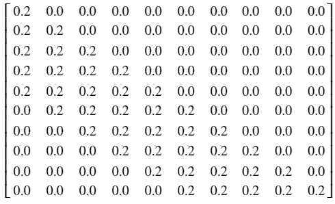
Figure 5: Truncated filter matrix
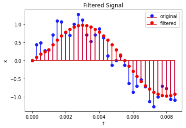
Figure 6: Original and filtered signal
DFT
The discrete Fourier transform (DFT) can likewise be represented as a matrix. Assuming an N-point DFT, the DFT matrix $W \in \mathbb{C}^{N \times N}$ has elements $w_{kl} = \dfrac{1}{\sqrt{N}} e^{-2 \pi j (k l) / N}$ where $k$ and $l$ are the rows and columns, respectively [1]. It is worth noting that $kl = kl \text{mod} N$ due to the circular convolution property of the DFT.
# construct DFT matrix
W = np.zeros((N, N), dtype=complex)
for k in range(N) :
    for l in range(N) :
        W[k, l] = np.exp(-2 * np.pi * 1j * (k * l) / N)

# DFT
X_w = W @ x

# get signal magnitude
w = fftfreq(N, 1/fs)[:N//2]
X_mag = 2 * np.abs(X_w[0:N//2]) / N

# plot results
plt.plot(w, X_mag)
plt.ylabel('Magnitude')
plt.xlabel('Frequency (Hz)')
plt.title('DFT of Signal')
plt.show()

Figure 7: Truncated DFT matrix
As can be seen below, the resulting magnitude plots line up with the frequency contents of the original signal $\mathbf{x}$.
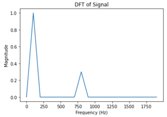
Figure 8: Frequencies of signal
Defining signal processing on graphs
In classical DSP, signals are either indexed temporally (such as audio), or spatially (such as an image). GSP extends this to indexes by nodes of a graph $\mathcal{G} = (\mathcal{V}, \mathcal{E}, W)$. This greatly increases the amount of problems that signal processing can be applied to, such as an unevenly spaced sensor network or social media interactions. Before, we said that an operator/transform on a signal can be represented by the matrix $A \in \mathbb{C}^{N \times N}$ and transformed by the equation $\mathbf{y} = A \mathbf{x}$. The matrix $A$ can take on a graphical representation by representing the adjacency matrix of a graph $\mathcal{G}$. [2]
Signals on graphs
Extending our signal model to graphs is fairly simple. Given a graph $\mathcal{G} = (\mathcal{V}, \mathcal{E}, W)$ with number of nodes $N = | \mathcal{V} |$, a signal is defined as $\mathbf{x} = [ x_0 \; x_1 \; … \; x_{N-1} ]^T$ where the value of the signal at node $n$ is given by $x_n$. [2]
Shifting with graphs
With this definiton of a graph signal in mind, we can define a shift in the graph domain as the movement of a value from one node to the next, defined on all nodes. The matrix (shown below) is very similar to the shift matrix defined here, with the only difference being that it “loops” back around. Viewing this from a graphical perspective, this is the adjacency matrix for a directed, cyclical graph. The adjacency matrix for this specific graph will henceforth be defined as $A_c \in \mathbb{R}^{N \times N}$. [2]
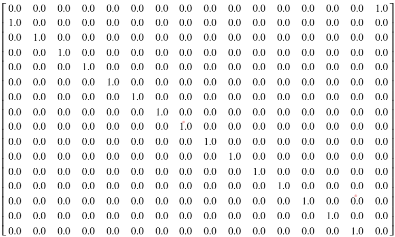
Figure 9: Graph Laplacian of cyclic shift graph
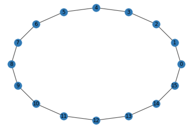
Figure 10: Displayed graph network of cyclic shift graph
It is important to note the role shift-invariance plays with this definition of a graph shift, and that this is not the only definition for it. Shift-invariance is a generalization of time-invariance, as defined for all discrete systems. A system $y(n) = h(n) x(n)$ is shift-invariant if, given a shift $x(n-k)$, the shift in the output $y(n-k)$ is equivalent to that of the input. In matrix notation, this is equivalent to the expression $AH = HA$ for a given matrix $A$. [2]
Filtering with graphs
Since our filter $H$ is shift-invariant, we can define $H$ as a polynomial of $A_c$ i.e. $H = h(A_c)$ with $h(\lambda_n) = h_0 + h_1 \lambda_n^1 + … + h_{M-1} \lambda_n^{M-1}$ for an $M$-order filter [3]. Using the eigendecomposition, we get the following:
$H = h(A) = h(U \Lambda U^{-1}) = U h(\Lambda ) U^{-1}$
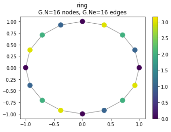
Below shows code for constructing our filter based off the cylic graph $A_c$. We first define a step function that restarts every 4 samples (i.e. a sawtooth wave with period of 4 samples) and a cyclic graph that’ll serve as the basis for our filter.
# define graph parameters
N = 16
x_step = np.arange(0, N)
x_osc = x_step % 4

# construct graph
G = graphs.Ring(N=N)

# display graph
G.plot_signal(x_osc)

Figure 11: Sawtooth signal on cyclic graph
We will next define our MA filter of size $L=2$. The graph filter is constructed as a polynomial of the graph adjacency’s eigenvalues as defined above. The graph filter matrix $H$ is then constructed from the modified eigenvalues.
# MA filter
L = 2
h = (1 / L) * np.ones(L)

# get eigens of adjacency
lamb, U = np.linalg.eig(A)

# transform eigenvalues with filter
h_lamb = np.zeros(N)
for n in range(N) :
    for i in range(L) :
        h_lamb[n] += h[i] * lamb[n] ** i

# construct filter
H = np.real(U @ np.diag(h_lamb) @ np.linalg.inv(U))

# apply filter
y_osc = H @ x_osc

# display result
G.plot_signal(y_osc)
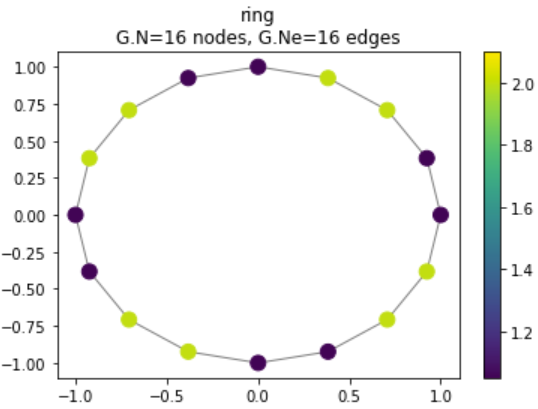
Figure 12: Lowpass filtered signal on cyclic graph
The result shows the filtered signal on the graph. Notice that, like the time-series MA filter, it smoothens the signal by filtering out high frequency contents.
DFT with graphs
Another interesting property of the cyclic graph with adjacency $A_c$ is that its eigenvalues are $e^{-j 2 \pi n / N}$ for $n=0, …, N-1$. Additionally, the ordered eigenvector matrix $U^{-1}$ of $A_c$ is equivalent to the DFT matrix defined in this section. Thus, we can construct a graph Fourier transform for a graph $\mathcal{G}$ and signal $\mathbf{x}$ with the following equation: $\mathbf{\hat{x}} = U^{-1} \mathbf{x}$, where $U^{-1}$ is computed using the eigendecomposition $A = U \Lambda U^{-1}$. [2]
# graph fourier transform
x_hat = np.abs(np.linalg.inv(U) @ x_osc)

# display result
G.plot_signal(x_hat)
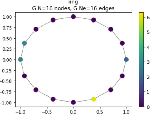
Figure 13: GFT of cyclic graph
The above code demonstrates the computation of the graph Fourier transform. Notice that the the highest magnitude node is the one corresponding to the fourth node down from the right-hand side, indicating a frequency of 4 samples (as defined before).
Conclusion
In this article, we have reviewed DSP concepts through the lense of linear algebra by defining common operators in the form of matrices. We then showed that a signal shifted on a cyclic graph is equivalent to shifting the signal in the time domain. Graphical filters are then constructed as polynomials of the graph adjacency, and the graph Fourier transform is shown to be the ordered matrix of eigenvectors of the graph adjacenecy. These methods all rely on the graph adjacenecy to define signal processing operators on graphs, which is useful for directed graphs. We will in the future use spectral graph methods to redefine many of these concepts to have have better numerical performance.
References
[1] Vetterli, Martin, Jelena Kovačević, and Vivek K. Goyal. Foundations of signal processing. Cambridge University Press, 2014.
[2] Ortega, Antonio, et al. “Graph signal processing: Overview, challenges, and applications.” Proceedings of the IEEE 106.5 (2018): 808-828.
[3] Stanković, Ljubiša, Miloš Daković, and Ervin Sejdić. “Introduction to graph signal processing.” Vertex-Frequency Analysis of Graph Signals. Springer, Cham, 2019. 3-108.
